Forest structure metrics extraction

Source: vignettes/forest.structure.metrics.Rmd

The R code below presents a forest structure metrics computation workflow from Airborne Laser Scanning (ALS) data. Workflow is based on functions from R packages lidaRtRee (tested with version 4.0.7) and lidR (tested with version 4.0.4). Package vegan is also required. Metrics are computed for each cell of a grid defined by a resolution. Those metrics are designed to describe the 3D structure of forest. Different types of metrics are computed:

1D height metrics,
2D metrics of the canopy height model (CHM),
tree segmentation metrics,
forest gaps and edges metrics.

The forest structure metrics derived from airborne laser scanning can be used for habitat suitability modelling and mapping. This workflow has been applied to compute the metrics used in the modeling and mapping of the habitat of Capercaillie (Tetrao urogallus)(Glad et al. (2020)), and those used for the modeling and mapping of a forest maturity index (Fuhr et al. (2022)). For more information about tree segmentation and gaps detection, please refer to the corresponding tutorials.

The workflow processes normalized point clouds provided as las/laz tiles of rectangular extent. Parallelization is used for faster processing, packages future and future.apply are used. A buffer is loaded around each tile to prevent border effects in tree segmentation and CHM processing.

Parameters

Set the number of cores to use for parallel computing.

# create parallel frontend, specify to use two parallel sessions
future::plan("multisession", workers = 2L)
# remove warning when using random numbers in parallel sessions
options(future.rng.onMisuse = "ignore")

Numerous parameters have to be set for processing.

# output metrics map resolution (m)
resolution <- 10
# canopy height model resolution (m)
res_chm <- 0.5
# buffer size (m) for tile processing (20 m is better for gaps metrics, 10 m is 
# enough for tree metrics)
buffer_size <- 20
# height threshold (m) for high points removal (points above this threshold are 
# considered as outliers)
points_max_h <- 60
# points classes to retain for analysis (vegetation + ground)
class_points <- c(0, 1, 2, 3, 4, 5)
# ground class
class_ground <- 2
# Gaussian filter sigma values in map units for multi-scale smoothing
sigma_l <- list(0, 0.5, 1, 2, 4, 8)
# fonction to computed raster statistics from multi-scale smoothing
smoothed_raster_stats <- function(x, mf) {
  data.frame(
    CHM0_sd = sd(x$smoothed_image_0),
    CHM0.5_sd = sd(x$smoothed_image_0.5),
    CHM1_sd = sd(x$smoothed_image_1),
    CHM2_sd = sd(x$smoothed_image_2),
    CHM4_sd = sd(x$smoothed_image_4),
    CHM8_sd = sd(x$smoothed_image_8),
    CHM_mean = mean(x$smoothed_image_0),
    CHM_PercInf0_5 = sum(x$smoothed_image_0 < 0.5) * mf,
    CHM_PercInf1 = sum(x$smoothed_image_0 < 1) * mf,
    CHM_PercSup5 = sum(x$smoothed_image_0 > 5) * mf,
    CHM_PercSup10 = sum(x$smoothed_image_0 > 10) * mf,
    CHM_PercSup20 = sum(x$smoothed_image_0 > 20) * mf,
    CHM_Perc1_5 = (sum(x$smoothed_image_0 < 5) - sum(x$smoothed_image_0 < 1)) *
      mf,
    CHM_Perc2_5 = (sum(x$smoothed_image_0 < 5) - sum(x$smoothed_image_0 < 2)) *
      mf
  )
}
# height breaks for penetration ratio and density
breaks_h <- c(-Inf, 0, 0.5, 1, 2, 5, 10, 20, 30, 60, Inf)
# percentiles of height distribution
percent <- c(0.10, 0.25, 0.5, 0.75, 0.9)
# surface breaks for gap size (m2)
breaks_gap_surface <- c(4, 16, 64, 256, 1024, 4096, Inf)
#
# gap surface names
n_breaks_gap <- gsub("-", "",
                     paste0("G_s",
                            breaks_gap_surface[c(-length(breaks_gap_surface))],
                            "to", breaks_gap_surface[c(-1)]
))
# height bin names
n_breaks_h <- gsub("-", "",
                   paste0("nb_H",
                          breaks_h[c(-length(breaks_h))], "to", breaks_h[c(-1)]
))
#

The first step is to create a catalog of LAS files (should be normalized, non-overlapping rectangular tiles). Preferably, tiles should be aligned on a multiple of resolution, and points should not lie on the northern or eastern border when such borders are common with adjacent tiles.

# create catalog of LAS files
cata <- lidR::readALSLAScatalog("./data/forest.structure.metrics")
# set coordinate system
lidR::projection(cata) <- 2154
# disable display of catalog processing
lidR::opt_progress(cata) <- FALSE
# option to read only xyzc attributes (coordinates, intensity, echo order and 
# classification) from height files (saves memory)
lidR::opt_select(cata) <- "xyzirnc"
# display
lidR::plot(cata, main = "Bounding box of las files")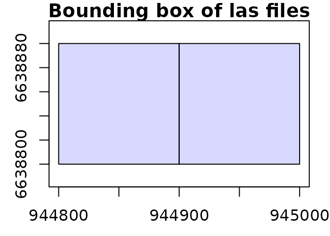

Workflow exemplified on one tile

Load point cloud

The tile is loaded, plus a buffer on adjacent tiles. Buffer points have a column “buffer” filled with 1.

# tile to process
i <- 1
# tile extent
b_box <- sf::st_bbox(cata[i,])
# load tile extent plus buffer
a <- lidR::clip_rectangle(
  cata, b_box[1] - buffer_size, b_box[2] - buffer_size, b_box[3] + buffer_size,
  b_box[4] + buffer_size
)
# add 'buffer' flag to points in buffer with TRUE value in this new attribute
a <- lidR::add_attribute(
  a, a$X < b_box[1] | a$Y < b_box[2] | a$X >= b_box[3] | a$Y >= b_box[4],
  "buffer"
)
a

## class        : LAS (v1.1 format 1)
## memory       : 14 Mb 
## extent       : 944800, 944920, 6638800, 6638900 (xmin, xmax, ymin, ymax)
## coord. ref.  : RGF93 v1 / Lambert-93 
## area         : 12000 m²
## points       : 333.3 thousand points
## density      : 27.77 points/m²
## density      : 14.46 pulses/m²

Only points from desired classes are retained. In case some mis-classified, high or low points remain in the data set, the point cloud is filtered and negative heights are replaced by 0.

# remove unwanted point classes, and points higher than height threshold
a <- lidR::filter_poi(a, is.element(Classification,
                                    class_points) & Z <= points_max_h)
# set negative heights to 0
a$Z[a$Z < 0] <- 0
#
summary(a@data)

##        X                Y                 Z           Intensity    
##  Min.   :944800   Min.   :6638800   Min.   : 0.00   Min.   :  2.0  
##  1st Qu.:944828   1st Qu.:6638825   1st Qu.: 2.33   1st Qu.: 27.0  
##  Median :944860   Median :6638850   Median : 9.94   Median : 67.0  
##  Mean   :944860   Mean   :6638849   Mean   :10.90   Mean   :101.7  
##  3rd Qu.:944891   3rd Qu.:6638872   3rd Qu.:18.14   3rd Qu.:135.0  
##  Max.   :944920   Max.   :6638900   Max.   :37.45   Max.   :821.0  
##   ReturnNumber   NumberOfReturns Classification    buffer       
##  Min.   :1.000   Min.   :1.000   Min.   :0.000   Mode :logical  
##  1st Qu.:1.000   1st Qu.:2.000   1st Qu.:5.000   FALSE:278011   
##  Median :1.000   Median :2.000   Median :5.000   TRUE :55218    
##  Mean   :1.713   Mean   :2.435   Mean   :4.122                  
##  3rd Qu.:2.000   3rd Qu.:3.000   3rd Qu.:5.000                  
##  Max.   :7.000   Max.   :7.000   Max.   :5.000

Canopy height model

The next step is to compute the canopy height model (CHM). It will be used to derive:

2D canopy height metrics related to multi-scale vertical heterogeneity (mean and standard deviation of CHM, smoothed at different scales)
tree metrics from tree top segmentation
gaps and edges metrics from gap segmentation

The CHM is computed and NA values are replaced by 0. A check is performed to make sure low or high points are not present.

# compute chm
chm <- lidR::rasterize_canopy(a, res = res_chm, algorithm = lidR::p2r(),
                              pkg = "terra")
# replace NA, low and high values
chm[is.na(chm) | chm < 0 | chm > points_max_h] <- 0
# display CHM
terra::plot(chm, main = "Canopy height model")

Metrics computation

2D CHM metrics

The CHM is smoothed with a Gaussian filter with different sigma values. Smoothed results are stored in a list and then integrated ito a single raster

# for each value in list of sigma, apply filtering to chm and store result in 
# list
st <- lapply(sigma_l, FUN = function(x) {
  lidaRtRee::dem_filtering(chm, nl_filter = "Closing", nl_size = 5,
                           sigma = x)$smoothed_image
})
# convert to raster
st <- terra::rast(st)
# modify layer names
names(st) <- paste0(names(st), "_", unlist(sigma_l))
# display
terra::plot(st, range = range(terra::values(st[[1]])))

The raster is then converted to points. Points outside the tile extent are removed and summary statistics (mean and standard deviation) of smoothed CHM heights are computed for each pixel at the output metrics resolution. Canopy covers in different height layers are also computed for the initial CHM after applying a non-linear filter designed to fill holes.

# crop to bbox
st <- terra::crop(st, terra::ext(b_box[1], b_box[3], b_box[2], b_box[4]))
# multiplying factor to compute proportion
mf <- 100 / (resolution / res_chm)^2

# compute raster metrics
metrics_2dchm <- lidaRtRee::raster_metrics(st,
                                           res = resolution,
                                           fun = function(x)
                                             smoothed_raster_stats(x, mf),
                                           output = "raster"
)
#
metrics_2dchm

## class       : SpatRaster 
## dimensions  : 10, 10, 14  (nrow, ncol, nlyr)
## resolution  : 10, 10  (x, y)
## extent      : 944800, 944900, 6638800, 6638900  (xmin, xmax, ymin, ymax)
## coord. ref. : RGF93 v1 / Lambert-93 (EPSG:2154) 
## source(s)   : memory
## names       :     CHM0_sd,   CHM0.5_sd,   CHM1_sd,   CHM2_sd,   CHM4_sd,   CHM8_sd, ... 
## min values  :  0.09293137,  0.08238094, 0.1268275, 0.2110724, 0.4235999, 0.1796814, ... 
## max values  : 11.99010774, 10.74751866, 9.4636706, 7.4926950, 4.2719578, 2.3223951, ...

Some outputs are displayed hereafter. On the first line are the standard deviation of CHM smoothed with different sigma values. On the second line are the CHM mean and percentages of CHM values below 1 m and above 10 m.

terra::plot(metrics_2dchm[[c(
  "CHM0_sd", "CHM1_sd", "CHM4_sd", "CHM_mean",
  "CHM_PercInf1", "CHM_PercSup10"
)]])

Gaps and edges metrics

Gaps are computed with the function gap_detection.

# compute gaps
gaps <- lidaRtRee::gap_detection(chm,
                                 ratio = 2, gap_max_height = 1,
                                 min_gap_surface = min(breaks_gap_surface),
                                 closing_height_bin = 1,
                                 nl_filter = "Median", nl_size = 3,
                                 gap_reconstruct = TRUE
)
# display maps
par(mfrow = c(1, 3))
terra::plot(chm, main = "CHM")
terra::plot(log(gaps$gap_surface), main = "Log of gap surface")
# display gaps
terra::plot(gaps$gap_id, main = "Gap id (random colors)",
            type = "classes", col = rainbow(8))#, legend = FALSE)

Summary statistics are then computed: pixel surface occupied by gaps in different size classes. Results are first cropped to the tile extent.

# crop results to tile size
gaps_surface <- terra::crop(gaps$gap_surface, terra::ext(
  b_box[1], b_box[3],
  b_box[2], b_box[4]
))
# compute gap statistics at final metrics resolution, in case gaps exist
if (!all(is.na(terra::values(gaps_surface)))) {
  metrics_gaps <- lidaRtRee::raster_metrics(gaps_surface,
                                            res = resolution,
                                            fun = function(x) {
                                              hist(x$gap_surface,
                                                   breaks = breaks_gap_surface,
                                                   plot = F
                                              )$counts * (res_chm / resolution)^2
                                            }, output = "raster"
  )
  # compute total gap proportion
  metrics_gaps$sum <- terra::tapp(metrics_gaps,
                                  rep(1, length(names(metrics_gaps))),
                                  fun = sum
  )
  # if gaps are present
  names(metrics_gaps) <- c(n_breaks_gap, paste("G_s", min(breaks_gap_surface),
                                               "toInf", sep = ""))
  # replace possible NA values by 0 (NA values are present in lines of the 
  # target raster
  # where no values >0 are present in the input raster)
  metrics_gaps[is.na(metrics_gaps)] <- 0
} else {
  metrics_gaps <- NULL
}
#
metrics_gaps

## class       : SpatRaster 
## dimensions  : 10, 10, 7  (nrow, ncol, nlyr)
## resolution  : 10, 10  (x, y)
## extent      : 944800, 944900, 6638800, 6638900  (xmin, xmax, ymin, ymax)
## coord. ref. : RGF93 v1 / Lambert-93 (EPSG:2154) 
## source(s)   : memory
## names       : G_s4to16, G_s16to64, G_s64to256, G_s256to1024, G_s10~o4096, G_s4096toInf, ... 
## min values  :    0.000,      0.00,     0.0000,            0,           0,            0, ... 
## max values  :    0.075,      0.32,     0.5175,            0,           1,            0, ...

Edges are detected with the function edge_detection as the outer envelope of the previously delineated gaps.

# Perform edge detection by erosion
edges <- lidaRtRee::edge_detection(gaps$gap_id > 0)
# display maps
par(mfrow = c(1, 3))
terra::plot(chm, main = "CHM")
terra::plot(gaps$gap_id > 0, main = "Gaps", legend = FALSE)
terra::plot(edges, main = "Edges", legend = FALSE)

The percentage of surface occupied by edges is then computed as summary statistic. Results are first cropped to the tile extent.

# crop results to tile size
edges <- terra::crop(
  edges,
  terra::ext(b_box[1], b_box[3], b_box[2], b_box[4])
)
# compute gap statistics at final metrics resolution, in case gaps exist
if (!all(is.na(terra::values(edges)))) {
  metrics_edges <- lidaRtRee::raster_metrics(edges,
                                             res = resolution,
                                             fun = function(x) {
                                               sum(x$lyr.1) *
                                                 (res_chm / resolution)^2
                                             }, output = "raster"
  )
  names(metrics_edges) <- "edges.proportion"
  # replace possible NA values by 0 (NA values are present in lines of the 
  # target raster where no values >0 are present in the input raster)
  metrics_edges[is.na(metrics_edges)] <- 0
} else {
  metrics_edges <- NULL
}
#
metrics_edges

## class       : SpatRaster 
## dimensions  : 10, 10, 1  (nrow, ncol, nlyr)
## resolution  : 10, 10  (x, y)
## extent      : 944800, 944900, 6638800, 6638900  (xmin, xmax, ymin, ymax)
## coord. ref. : RGF93 v1 / Lambert-93 (EPSG:2154) 
## source(s)   : memory
## name        : edges.proportion 
## min value   :           0.0000 
## max value   :           0.1225

Some outputs are displayed hereafter. The proportion of surface occupied by gaps of various sizes is depicted as well as the proportion of surface occupied by edges.

par(mfrow = c(1, 3))
# terra::plot(metrics_gaps[["G_s4to16"]], main="Prop of gaps 4-16m2")
terra::plot(metrics_gaps[["G_s64to256"]], main = "Prop of gaps 64-256m2")
terra::plot(metrics_gaps[["G_s4toInf"]], main = "Prop of gaps >4m2")
terra::plot(metrics_edges, main = "Proportion of edges")

Tree metrics

Tree tops are detected with the function treeSegmentation and then extracted with treeExtraction.

# tree top detection (default parameters)
segms <- lidaRtRee::tree_segmentation(chm, hmin = 5)
# extraction to data.frame
trees <- lidaRtRee::tree_extraction(segms)
# display maps
par(mfrow = c(1, 2))
terra::plot(chm, main = "CHM and tree tops")
points(trees$x, trees$y, pch = 4, cex = 0.3)
# display segments, except ground segment
dummy <- segms$segments_id
dummy[dummy == 0] <- NA
terra::plot(dummy, main = "Segments (random colors)",
            col = rainbow(8), type = "classes", legend = FALSE)
points(trees$x, trees$y, pch = 4, cex = 0.3)

Results are cropped to the tile extent. Summary statistics from std_tree_metrics are then computed for each pixel. Canopy cover in trees and mean canopy height in trees are computed in a second step because they can not be computed from the data of the extracted trees which crowns may span several output pixels. They are calculated from the images obtained during the previous tree segmentation.

# remove trees outside of tile
trees <- trees[trees$x >= b_box[1] & trees$x < b_box[3] & trees$y >= b_box[2] & 
                 trees$y < b_box[4], ]
# compute raster metrics
metrics_trees <- 
  lidaRtRee::raster_metrics(trees[, -1],
                            res = resolution,
                            fun = function(x) {
                              lidaRtRee::std_tree_metrics(x,
                                                          resolution^2 / 10000)
                            }, output = "raster"
  )
# remove NAs and NaNs
metrics_trees[!is.finite(metrics_trees)] <- 0
#
# compute canopy cover in trees and canopy mean height in trees
# in region of interest, because it is not in previous step.
r_tree_chm <- segms$filled_dem
# set chm to NA in non segment area
r_tree_chm[segms$segments_id == 0] <- NA
# compute raster metrics
dummy <- lidaRtRee::raster_metrics(terra::crop(
  r_tree_chm,
  terra::ext(
    b_box[1], b_box[3], b_box[2],
    b_box[4]
  )
),
res = resolution,
fun = function(x) {
  c(
    sum(!is.na(x$filled_dem)) / (resolution / res_chm)^2,
    mean(x$filled_dem, na.rm = T)
  )
},
output = "raster"
)
names(dummy) <- c("TreeCanopy_cover_in_plot", "TreeCanopy_meanH_in_plot")
#
dummy <- terra::extend(dummy, metrics_trees)
metrics_trees <- c(metrics_trees, dummy)
#
metrics_trees

## class       : SpatRaster 
## dimensions  : 10, 10, 13  (nrow, ncol, nlyr)
## resolution  : 10, 10  (x, y)
## extent      : 944800, 944900, 6638800, 6638900  (xmin, xmax, ymin, ymax)
## coord. ref. : RGF93 v1 / Lambert-93 (EPSG:2154) 
## source(s)   : memory
## names       : Tree_meanH, Tree_sdH, Tree_giniH, Tree_density, TreeI~nsity, TreeS~nsity, ... 
## min values  :       0.00,  0.00000,  0.0000000,            0,           0,           0, ... 
## max values  :      37.18, 15.19572,  0.2050181,          500,         200,         500, ...

Some outputs are displayed hereafter.

par(mfrow = c(1, 3))
terra::plot(metrics_trees$Tree_meanH, main = "Mean (detected) tree height (m)")
points(trees$x, trees$y, cex = trees$h / 40)
terra::plot(metrics_trees$TreeSup20_density,
             main = "Density of (detected) trees > 20m (/ha)"
)
terra::plot(metrics_trees$Tree_meanCrownVolume,
             main = "Mean crown volume of detected trees (m3)"
)

Point cloud (1D) metrics

Buffer points are first removed from the point cloud, then metrics are computed from all points and from vegetation points only.

# remove buffer points
a <- lidR::filter_poi(a, buffer == 0)
#
# all points metrics
metrics_1d <- lidR::pixel_metrics(a, as.list(c(
  as.vector(quantile(Z, probs = percent)),
  sum(Classification == 2),
  mean(Intensity[ReturnNumber == 1])
)), res = resolution)
names(metrics_1d) <- c(paste("Hp", percent * 100, sep = ""),
                       "nb_ground", "Imean_1stpulse")
#
# vegetation-only metrics
a <- lidR::filter_poi(a, Classification != class_ground)
dummy <- lidR::pixel_metrics(a, as.list(c(
  mean(Z),
  max(Z),
  sd(Z),
  length(Z),
  hist(Z, breaks = breaks_h, right = F, plot = F)$counts
)), res = resolution)
names(dummy) <- c("Hmean", "Hmax", "Hsd", "nb_veg", n_breaks_h)
# merge rasterstacks
dummy <- terra::extend(dummy, metrics_1d)
metrics_1d <- c(metrics_1d, dummy)
rm(dummy)
# crop to tile extent
metrics_1d <- terra::crop(metrics_1d,
                          terra::ext(b_box[1], b_box[3], b_box[2], b_box[4]))

Based on those metrics, additional metrics are computed (Simpson index, relative density in height bins and penetration ratio in height bins)

# Simpson index
metrics_1d$Hsimpson <- terra::app(
  metrics_1d[[n_breaks_h[c(-1, -length(n_breaks_h))]]],
  function(x, ...) {
    vegan::diversity(x, index = "simpson")
  }
)
# Relative density 
for (i in n_breaks_h[c(-1, -length(n_breaks_h))])
{
  metrics_1d[[gsub("nb", "relativeDensity", i)]] <-
    metrics_1d[[i]] / (metrics_1d$nb_veg + metrics_1d$nb_ground)
}
# Penetration ratio
# cumulative sum
cumu_sum <- metrics_1d[["nb_ground"]]
for (i in n_breaks_h)
{
  cumu_sum <- c(cumu_sum, cumu_sum[[dim(cumu_sum)[3]]] + metrics_1d[[i]])
}
names(cumu_sum) <- c("nb_ground", n_breaks_h)
# compute interception ratio of each layer
intercep_ratio <- cumu_sum[[-1]]
for (i in 2:dim(cumu_sum)[3])
{
  intercep_ratio[[i - 1]] <- 1 - cumu_sum[[i - 1]] / cumu_sum[[i]]
}
names(intercep_ratio) <- gsub("nb", "intercepRatio", names(cumu_sum)[-1])
# merge rasterstacks
metrics_1d <- c(metrics_1d, intercep_ratio)
# rm(cumu_sum, intercep_ratio)
#
metrics_1d

## class       : SpatRaster 
## dimensions  : 10, 10, 40  (nrow, ncol, nlyr)
## resolution  : 10, 10  (x, y)
## extent      : 944800, 944900, 6638800, 6638900  (xmin, xmax, ymin, ymax)
## coord. ref. : RGF93 v1 / Lambert-93 (EPSG:2154) 
## source(s)   : memory
## names       :  Hp10,  Hp25,   Hp50,  Hp75,  Hp90, nb_ground, ... 
## min values  :  0.00,  0.00,  0.010,  0.03,  0.06,        52, ... 
## max values  : 17.62, 22.69, 25.725, 27.91, 31.67,       982, ...

Some outputs are displayed hereafter.

# display results
par(mfrow = c(1, 3))
terra::plot(metrics_1d$Imean_1stpulse, main = "Mean intensity (1st return)")
terra::plot(metrics_1d$Hp50, main = "Percentile 50 of heights")
terra::plot(metrics_1d$intercepRatio_H2to5, main = "Interception ratio 2-5 m")

Batch processing

The following code uses parallel processing to handle multiple files of a catalog, and arranges all metrics in a raster. Code in the Parameters section has to be run beforehand.

# processing by tile
metrics <- future.apply::future_lapply(
  as.list(1:nrow(cata)),
  FUN = function(i) {
    # tile extent
    b_box <- sf::st_bbox(cata[i,])
    # load tile extent plus buffer
    a <- try(lidR::clip_rectangle(
      cata,
      b_box[1] - buffer_size,
      b_box[2] - buffer_size,
      b_box[3] + buffer_size,
      b_box[4] + buffer_size
    ))
    #
    # check if points are successfully loaded
    if (class(a) == "try-error") {
      return(NULL)
    }
    # add 'buffer' flag to points in buffer with TRUE value in this new attribute
    a <- lidR::add_attribute(a,
                             a$X < b_box[1] | a$Y < b_box[2] | 
                               a$X >= b_box[3] | a$Y >= b_box[4],
                             "buffer")
    # remove unwanted point classes, and points higher than height threshold
    a <-
      lidR::filter_poi(a,
                       is.element(Classification,
                                  class_points) & Z <= points_max_h)
    # check number of remaining points
    if (nrow(a) == 0)
      return(NULL)
    # set negative heights to 0
    a$Z[a$Z < 0] <- 0
    #
    # compute chm
    chm <- lidR::rasterize_canopy(a, res = res_chm, algorithm = lidR::p2r(),
                                  pkg = "terra")
    # replace NA, low and high values
    chm[is.na(chm) | chm < 0 | chm > points_max_h] <- 0
    #-----------------------
    # compute 2D CHM metrics
    # for each value in list of sigma, apply filtering to chm and store result 
    # in list
    st <- lapply(
      sigma_l,
      FUN = function(x) {
        lidaRtRee::dem_filtering(chm,
                                 nl_filter = "Closing",
                                 nl_size = 5,
                                 sigma = x)$smoothed_image
      }
    )
    # convert to raster
    st <- terra::rast(st)
    # modify layer names
    names(st) <- paste0(names(st), "_", unlist(sigma_l))
    # crop to bbox
    st <-
      terra::crop(st, terra::ext(b_box[1], b_box[3], b_box[2], b_box[4]))
    # multiplying factor to compute proportion
    mf <- 100 / (resolution / res_chm) ^ 2
    # compute raster metrics
    metrics_2dchm <-
      lidaRtRee::raster_metrics(
        st,
        res = resolution,
        fun = function(x) smoothed_raster_stats(x, mf),
        output = "raster"
      )
    #
    # -------------------
    # compute gap metrics
    gaps <- lidaRtRee::gap_detection(
      chm,
      ratio = 2,
      gap_max_height = 1,
      min_gap_surface = min(breaks_gap_surface),
      closing_height_bin = 1,
      nl_filter = "Median",
      nl_size = 3,
      gap_reconstruct = TRUE
    )
    # crop results to tile size
    gaps_surface <- terra::crop(gaps$gap_surface,
                                 terra::ext(b_box[1], b_box[3], b_box[2],
                                                b_box[4]))
    # compute gap statistics at final metrics resolution, in case gaps exist
    if (!all(is.na(terra::values(gaps_surface)))) {
      metrics_gaps <- lidaRtRee::raster_metrics(
        gaps_surface,
        res = resolution,
        fun = function(x) {
          hist(x$gap_surface,
               breaks = breaks_gap_surface,
               plot = F)$counts * (res_chm / resolution) ^
            2
        },
        output = "raster"
      )
      # compute total gap proportion
      metrics_gaps$sum <- terra::tapp(metrics_gaps,
                                      rep(1, length(names(metrics_gaps))),
                                      fun = sum
      )
      # if gaps are present
      names(metrics_gaps) <-
        c(n_breaks_gap, paste("G_s", min(breaks_gap_surface), "toInf",
                              sep = ""))
      # replace possible NA values by 0 (NA values are present in lines of the 
      # target raster where no values >0 are present in the input raster)
      metrics_gaps[is.na(metrics_gaps)] <- 0
    } else {
      metrics_gaps <- NULL
    }
    #
    # --------------------
    # compute edge metrics
    # Perform edge detection by erosion
    edges <- lidaRtRee::edge_detection(gaps$gap_id > 0)
    # crop results to tile size
    edges <- terra::crop(edges, terra::ext(b_box[1], b_box[3],
                                                b_box[2], b_box[4]))
    # compute edges statistics at final metrics resolution, in case edges exist
    if (!all(is.na(terra::values(edges)))) {
      metrics_edges <- lidaRtRee::raster_metrics(
        edges,
        res = resolution,
        fun = function(x) {
          sum(x$lyr.1) * (res_chm / resolution) ^ 2
        },
        output = "raster"
      )
      names(metrics_edges) <- "edges.proportion"
      # replace possible NA values by 0 (NA values are present in lines of the 
      # target raster where no values >0 are present in the input raster)
      metrics_edges[is.na(metrics_edges)] <- 0
    } else {
      metrics_edges <- NULL
    }
    #
    # --------------------
    # compute tree metrics
    # tree top detection (default parameters)
    segms <- lidaRtRee::tree_segmentation(chm, hmin = 5)
    # extraction to data.frame
    trees <-
      lidaRtRee::tree_extraction(segms$filled_dem, segms$local_maxima,
                                 segms$segments_id)
    # remove trees outside of tile
    trees <-
      trees[trees$x >= b_box[1] &
              trees$x < b_box[3] & trees$y >= b_box[2] & trees$y < b_box[4],]
    # compute raster metrics
    metrics_trees <- lidaRtRee::raster_metrics(
      trees[,-1],
      res = resolution,
      fun = function(x) {
        lidaRtRee::std_tree_metrics(x, resolution ^ 2 / 10000)
      },
      output = "raster"
    )
    # remove NAs and NaNs
    metrics_trees[!is.finite(metrics_trees)] <- 0
    #
    # extend layer in case there are areas without trees
    metrics_trees <-
      terra::extend(metrics_trees, metrics_2dchm)
    # set NA values to 0
    metrics_trees[is.na(metrics_trees)] <- 0
    # compute canopy cover in trees and canopy mean height in trees
    # in region of interest, because it is not in previous step.
    r_tree_chm <- segms$filled_dem
    # set chm to NA in non segment area
    r_tree_chm[segms$segments_id == 0] <- NA
    # compute raster metrics
    dummy <- lidaRtRee::raster_metrics(
      terra::crop(r_tree_chm, terra::ext(b_box[1], b_box[3], b_box[2],
                                         b_box[4])),
      res = resolution,
      fun = function(x) {
        c(sum(!is.na(x$filled_dem)) / (resolution / res_chm) ^ 2,
          mean(x$filled_dem, na.rm = T))
      },
      output = "raster"
    )
    names(dummy) <-
      c("TreeCanopy_cover_in_plot", "TreeCanopy_meanH_in_plot")
    dummy <- terra::extend(dummy, metrics_2dchm)
    # set NA values to 0
    dummy[is.na(dummy)] <- 0
    #
    metrics_trees <-c(metrics_trees, dummy)
    #
    # -------------------------
    # compute 1D height metrics
    # remove buffer points
    a <- lidR::filter_poi(a, buffer == 0)
    #
    if (nrow(a) == 0) {
      metrics_1d <- NULL
    } else {
      # all points metrics
      metrics_1d <- lidR::pixel_metrics(a, as.list(c(
        as.vector(quantile(Z, probs = percent)),
        sum(Classification == 2),
        mean(Intensity[ReturnNumber == 1])
      )), res = resolution)
      names(metrics_1d) <-
        c(paste("Hp", percent * 100, sep = ""),
          "nb_ground",
          "Imean_1stpulse")
      #
      # vegetation-only metrics
      a <- lidR::filter_poi(a, Classification != class_ground)
      if (nrow(a) != 0) {
        dummy <- lidR::pixel_metrics(a, as.list(c(
          mean(Z),
          max(Z),
          sd(Z),
          length(Z),
          hist(
            Z,
            breaks = breaks_h,
            right = F,
            plot = F
          )$counts
        )), res = resolution)
        names(dummy) <-
          c("Hmean", "Hmax", "Hsd", "nb_veg", n_breaks_h)
        # merge raster
        dummy <- terra::extend(dummy, metrics_1d)
        metrics_1d <- c(metrics_1d, dummy)
        rm(dummy)
        # -------------
        # merge metrics
        metrics_1d <-
          terra::extend(metrics_1d, metrics_2dchm)
        # metrics_1d[is.na(metrics_1d)] <- 0
        metrics_1d <- terra::crop(metrics_1d, metrics_2dchm)
        metrics_gaps <-
          terra::extend(metrics_gaps, metrics_2dchm)
        # metrics_gaps[is.na(metrics_gaps)] <- 0
        metrics_gaps <- terra::crop(metrics_gaps, metrics_2dchm)
        metrics_edges <-
          terra::extend(metrics_edges, metrics_2dchm)
        # metrics_edges[is.na(metrics_edges)] <- 0
        metrics_edges <- terra::crop(metrics_edges, metrics_2dchm)
        metrics_trees <- terra::crop(metrics_trees, metrics_2dchm)
        #
        temp <- c(metrics_1d,
                                 metrics_2dchm,
                                 metrics_gaps,
                                 metrics_edges,
                                 metrics_trees)
        temp[is.na(temp)] <- 0
      } # end of vegetation-only points presence check
    } # end of buffer-less points presence check
    return(terra::wrap(temp))
  }
)
# --------------
# mosaic rasters
# unpack rasters
metrics <- lapply(metrics, terra::rast)
# names_metrics <- names(metrics[[1]])
metrics <- do.call(terra::merge, metrics)
# names(metrics) <- names_metrics
# --------------------------
# compute additional metrics
# Simpson index
metrics$Hsimpson <- terra::app(metrics[[n_breaks_h[c(-1,-length(n_breaks_h))]]],
                                       function(x, ...) {
                                         vegan::diversity(x, index = "simpson")
                                       })
#
# Relative density
for (i in n_breaks_h[c(-1,-length(n_breaks_h))])
{
  metrics[[gsub("nb", "relativeDensity", i)]] <-
    metrics[[i]] / (metrics$nb_veg + metrics$nb_ground)
}
# Penetration ratio
# compute cumulative sum
cumu_sum <- metrics[["nb_ground"]]
for (i in n_breaks_h)
{
  cumu_sum <-
    c(cumu_sum, cumu_sum[[dim(cumu_sum)[3]]] + metrics[[i]])
}
names(cumu_sum) <- c("nb_ground", n_breaks_h)
# interception ratio
intercep_ratio <- cumu_sum[[-1]]
for (i in 2:dim(cumu_sum)[3])
{
  intercep_ratio[[i - 1]] <- 1 - cumu_sum[[i - 1]] / cumu_sum[[i]]
}
names(intercep_ratio) <- gsub("nb", "intercepRatio", names(cumu_sum)[-1])
# merge rasterstacks
metrics <- c(metrics, intercep_ratio)
#
# ----------------------
# export as raster files
# for (i in 1:names(metrics))
# {
#  print(i)
#  writeRaster(metrics[[i]],
# file=paste("output/raster_",i,"_",resolution,"m.tif",sep="")
# }
# -------
# display
terra::plot(metrics[[c("Imean_1stpulse", "Hsimpson")]],
             main = c("Mean intensity of 1st pulse",
                      "Simpson indice of point heights")
)

References

Fuhr, Marc, Etienne Lalechère, Jean-Matthieu Monnet, and Laurent Bergès. 2022. “Detecting Overmature Forests with Airborne Laser Scanning (ALS).” Remote Sensing in Ecology and Conservation 8 (5): 731–43. https://doi.org/https://doi.org/10.1002/rse2.274.

Glad, Anouk, Björn Reineking, Marc Montadert, Alexandra Depraz, and Jean-Matthieu Monnet. 2020. “Assessing the Performance of Object-Oriented LiDAR Predictors for Forest Bird Habitat Suitability Modeling.” Remote Sensing in Ecology and Conservation 6 (1): 5–19. https://doi.org/10.1002/rse2.117.

Jean-Matthieu Monnet, with contributions from B. Reineking and A. Glad